Centennial Job Corps Students Support Firefighting Preparedness through Camp Crew

Centennial Job Corps camp crew cleaning hose

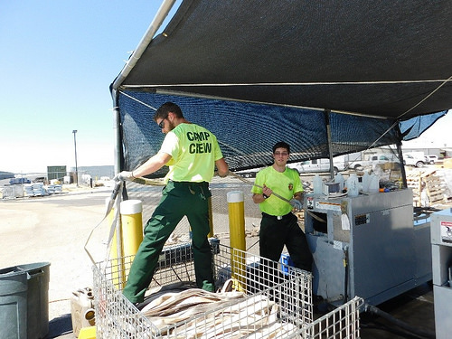
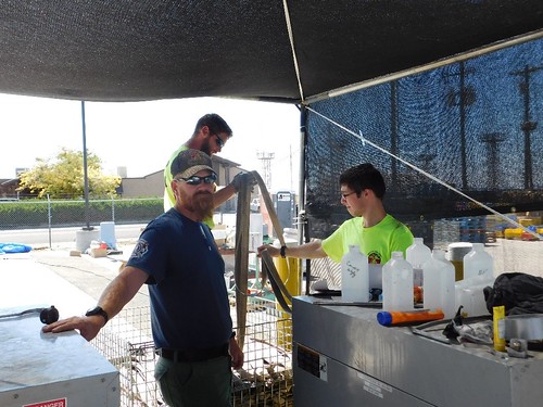
Centennial Job Corps camp crew cleaning hose returned from the fire line. Forest Service photo

In the back parking lot of the National Interagency Fire Center (NIFC), seven workers wear neon green shirts with the Camp Crew logo written across the back.

And they stand out.

They are young and their bright T-shirts contrast with those of the more seasoned personnel. As the crew works among large mounds of fire hose spread throughout the lot, it’s obvious they have one thing on their mind: meticulously preparing the hose for the next fire.

As the camp crew works to support the fire operations, military veteran Loren VanHorn supports them as the Camp Crew Boss.

Five years ago, VanHorn was exploring retirement options after serving 20 years in the military when a former supervisor and friend mentioned the Centennial Job Corps in Nampa, Idaho.  He’s been with Centennial ever since.

Centennial Job Corps’ Loren VanHorn

Centennial Job Corps’ Loren VanHorn leads a Camp Crew at the National Interagency Fire Center. Forest Service photo

“My job and goal is to prepare and mentor these students for the challenges of fire support assignments, working in a stressful environment as a team, and supporting them in-part with the skill sets I learned in the military: leadership, honor and a work ethic,” VanHorn said.

For the 2016 fire season, the Boise National Forest worked with the Center to hire four retired military veterans to oversee two Camp Crews consisting of ten students each. These veterans bring command presence, leadership, solid work ethic and the ability to make decisions under stress. They serve as excellent student mentors for future career ambitions.

The Centennial Job Corps program has several trade programs for all students including carpentry, welding and nursing. Camp Crews also work at Incident Command Posts providing support to the logistic sections and have even helped radio technicians on incidents.

Centennial Job Corps drying fire hose

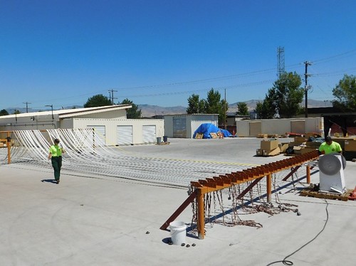
Centennial Job Corps drying fire hose in preparation for the next fire. Forest Service photo

Forest Service Centennial Job Corps Assistant Fire Management Officer, Mike Towers says that students in the Job Corps Fire Program are looked up to by the Centennial student body.

“They all know that their peers who volunteer for the program demonstrate integrity, solid work ethics, making decisions under stress, and serve as excellent mentors,” said Towers. “Having retired veterans is an added bonus and we are very fortunate to have them as Camp Crew Bosses.”

“I am extremely proud of all of these students and veterans and their contribution to the success of the Centennial Job Corps Camp Crews,” Towers said. “Together they are a testament to hard work, determination, with a willingness to succeed and are the true back bone to the success of the Centennial Job Corps camp crews.”

Because September is National Preparedness Month, it is a good time to think about emergency planning.  Don’t Wait. Communicate. Make an Emergency Communication Plan for you and your family because you just don’t know when disasters will impact your community.

Used fire house at the Pioneer Fire

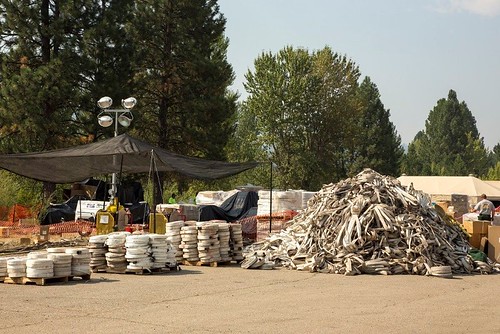
Used fire house at the Pioneer Fire. Forest Service photo

The Annual Harvest Challenge: Student Teams Supported by Chefs Move to Schools and Farm to School

Cross-posted from the Let’s Move blog:

The annual Harvest Challenge, menu planning and cooking event for high school students, is an important example of how aspiring chefs get started and learn to create winning recipes.

This exciting contest, which is now going into its 8th year, challenges teams of high school students – including staff and chef mentors – to develop a creative, appetizing and visually appealing school lunch entrée and side dish while incorporating locally grown foods. At the same time, the entrée and side dish must comply with USDA National School Lunch nutrition standards and meet a budget of $1 per person per serving (entrée and side dish combined). “This is a fun and challenging event for our high school students that really enables them to appreciate the hard work that goes into school food programs,” says Ashlee Gabrielson, director of the Vernon County Farm to School Program in Wisconsin.

At the 7th annual Harvest Challenge event sponsored by the Vernon County Farm to School Program, USDA Deputy Under Secretary for Food, Nutrition and Consumer Services, Dr. Katie Wilson, served as a speaker and celebrity judge. There, she presented the winning awards and said, “Thank you to all who dedicate their time and energy to Farm to School and the Chefs Move to Schools Initiative throughout the school year.”

In a very close competition, six Wisconsin school districts were represented in 2015. Hillsboro High School aspiring chefs won the judge’s choice by a single vote, taking home the traveling trophy with their delicious Italian BBQ and Corn. Viroqua High School won for student choice, with their tasty breakfast taco, cinnamon sugar chips, and spicy fruit salsa; and Kickapoo High School took home the community choice vote by preparing harvest chili and pumpkin muffins. We can’t wait to see what they cook up for 2016!

The Harvest Challenge seeks to create healthier students and stronger rural economies by linking school food service programs with local food producers. The Challenge highlights the many delicious benefits of fresh and nutritious local foods in school lunch programs. We encourage schools across the country to partner with their local Farm to School program and host their own Harvest Challenge this fall!

This is yet another activity that highlights how chefs and schools are working together to engage youth about food in a fun and appealing way. As a part of First Lady Michelle Obama’s Let’s Move! initiative, Chefs Move to Schools seeks to utilize the creativity and culinary expertise of chefs to help schools ensure that America’s youngest generation grows up healthy. Chefs nationwide are lending their creativity and skills to assist in schools’ efforts in the classroom, cafeteria, and culinary trainings/demonstrations.

Chefs interested in volunteering with Chefs Move to Schools and partner with schools in their area can register at Chefs Move to Schools.  Schools can also find a local chef volunteer using the chef locator tool.

The Snyder Sensitivity Situation

Nature published a great new reconstruction of global temperatures over the past 2 million years today. Snyder (2016) uses 61 temperature reconstructions from 59 globally diverse sediment cores and a correlation structure from model simulations of the last glacial maximum to estimate (with uncertainties) the history of global temperature back through the last few dozen ice ages cycles. There are multiple real things to discuss about this – the methodology, the relatively small number of cores being used (compared to what could have been analyzed), the age modeling etc. – and many interesting applications – constraints on polar amplification, the mid-Pleistocene transition, the duration and nature of previous interglacials – but unfortunately, the bulk of the attention will be paid to a specific (erroneous) claim about Earth System Sensitivity (ESS) that made it into the abstract and was the lead conclusion in the press release.

The paper claims that ESS is ~9ºC and that this implies that the long term committed warming from today’s CO2 levels is a further 3-7ºC. This is simply wrong.


The Snyder (2016) reconstruction of global temperatures compared to Antarctic ice core temperature and CO2, and deep water temperatures.

I recently posted a summary of why you can’t constrain ‘Earth System Sensitivity’ (the long term response of the climate system, including ice sheets, vegetation etc.) just by looking at the regression between the forcing from CO2 (and other greenhouse gases) over the ice age cycles. That regression has been looked at before, and Snyder (2016) updates that with her new (and slightly higher amplitude) temperature reconstruction. Unfortunately, she then associates this regression with the Earth System Sensitivity (which it is not) to get a value of ~9ºC for a doubling of CO2.

In the previous post, I outlined how the combination of carbon cycle feedbacks to the Milankovitch forcing and the climate system response to CO2 gives rise to this correlation and that – by itself – it can’t be used to define the latter term. Furthermore, because the regression is being defined over ice age cycles where the biggest changes are related to the (now disappeared) North American and Fenno-Scandanavian ice sheets, the regression might well be much less for situations where only Greenland and West Antarctica are “in play”.

So, what do we think the ESS is, and how does that impact our view of committed warming today? There have been a few papers on this; Hansen et al (2008), Lunt et al (2010) and Palaeosens (2012). They have focused on looking at the warmer climates of the Cenozoic (the Pliocene, etc.) to avoid the confusion from the response of ice sheets to orbital forcing during the ice age cycles of the Pleistocene, but obviously have significant uncertainties due to less precision about ancient greenhouse gas levels. The ESS values range from about 4.5ºC to 6ºC for a doubling of CO2. One other study came up with substantially higher numbers derived from the PETM (Pagani et al, 2010), but a number of assumptions made there limit it’s applicability to today’s climate.

The current energy imbalance (just a little less than 1 W/m2) implies that the planet would need to warm by ~ 1 x S / 3.7 ºC to restore an equilibrium, and using the standard climate sensitivity of 3ºC for a doubling of CO2, implies a committed warming of 0.8ºC or so. To leap from that to the claimed 3-7ºC warming requires that the changes in the ice sheets and vegetation arising from the current and (medium term) committed warming would increase the radiative imbalance by another ~2 W/m2 – and that is extreme (for reference, the changes between the last ice age and now from these factors is only about 4 W/m2 (Kohler et al, 2010) with the huge impact of the N. American and European ice sheets included).

Thus, Snyder’s claim of a committed warming of 3-7ºC is based on an incorrect method for defining ESS, an inappropriate application of this to the present and is inconsistent with current estimates of the radiative imbalance and plausible future changes in ice sheets.

For clarification, this is not an argument about what ESS is, nor is it a claim that we should ignore the long-term responses of the system to current forcing, nor does it mean that paleoclimate has nothing to tell us about future changes (au contraire!). The objection I have is only to this very specific calculation and its subsequent application.

I don’t want to speculate on how this situation can have occurred. However the maxim that “extraordinary claims require extraordinary evidence” suggests that it might have behoved the editors to require further checks of such a dramatic statement before going to press. As it is, many will claim that this is yet another example of a high profile journal going for press attention over rigourous science. The net result of the conflicting media reports and criticism will likely be a greater confusion about the relevant science, and an overshadowing of what is at heart a good contribution to understanding climate history and that is a shame.

References


  1. C.W. Snyder, “Evolution of global temperature over the past two million years”, Nature, 2016. http://dx.doi.org/10.1038/nature19798


  2. V. Masson-Delmotte, B. Stenni, K. Pol, P. Braconnot, O. Cattani, S. Falourd, M. Kageyama, J. Jouzel, A. Landais, B. Minster, J. Barnola, J. Chappellaz, G. Krinner, S. Johnsen, R. Röthlisberger, J. Hansen, U. Mikolajewicz, and B. Otto-Bliesner, “EPICA Dome C record of glacial and interglacial intensities”, Quaternary Science Reviews, vol. 29, pp. 113-128, 2010. http://dx.doi.org/10.1016/j.quascirev.2009.09.030


  3. J. Hansen, M. Sato, P. Kharecha, D. Beerling, R. Berner, V. Masson-Delmotte, M. Pagani, M. Raymo, D.L. Royer, and J.C. Zachos, “Target Atmospheric CO2: Where Should Humanity Aim?”, TOASCJ, vol. 2, pp. 217-231, 2008. http://dx.doi.org/10.2174/1874282300802010217


  4. D.J. Lunt, A.M. Haywood, G.A. Schmidt, U. Salzmann, P.J. Valdes, and H.J. Dowsett, “Earth system sensitivity inferred from Pliocene modelling and data”, Nature Geoscience, vol. 3, pp. 60-64, 2009. http://dx.doi.org/10.1038/NGEO706


  5. E.J. Rohling, E.J. Rohling, A. Sluijs, H.A. Dijkstra, P. Köhler, R.S.W. van de Wal, A.S. von der Heydt, D.J. Beerling, A. Berger, P.K. Bijl, M. Crucifix, R. DeConto, S.S. Drijfhout, A. Fedorov, G.L. Foster, A. Ganopolski, J. Hansen, B. Hönisch, H. Hooghiemstra, M. Huber, P. Huybers, R. Knutti, D.W. Lea, L.J. Lourens, D. Lunt, V. Masson-Demotte, M. Medina-Elizalde, B. Otto-Bliesner, M. Pagani, H. Pälike, H. Renssen, D.L. Royer, M. Siddall, P. Valdes, J.C. Zachos, and R.E. Zeebe, “Making sense of palaeoclimate sensitivity”, Nature, vol. 491, pp. 683-691, 2012. http://dx.doi.org/10.1038/nature11574


  6. M. Pagani, Z. Liu, J. LaRiviere, and A.C. Ravelo, “High Earth-system climate sensitivity determined from Pliocene carbon dioxide concentrations”, Nature Geoscience, vol. 3, pp. 27-30, 2009. http://dx.doi.org/10.1038/NGEO724


  7. P. Köhler, R. Bintanja, H. Fischer, F. Joos, R. Knutti, G. Lohmann, and V. Masson-Delmotte, “What caused Earth’s temperature variations during the last 800,000 years? Data-based evidence on radiative forcing and constraints on climate sensitivity”, Quaternary Science Reviews, vol. 29, pp. 129-145, 2010. http://dx.doi.org/10.1016/j.quascirev.2009.09.026


  8. G.A. Schmidt, J.D. Annan, P.J. Bartlein, B.I. Cook, E. Guilyardi, J.C. Hargreaves, S.P. Harrison, M. Kageyama, A.N. LeGrande, B. Konecky, S. Lovejoy, M.E. Mann, V. Masson-Delmotte, C. Risi, D. Thompson, A. Timmermann, L. Tremblay, and P. Yiou, “Using palaeo-climate comparisons to constrain future projections in CMIP5”, Climate of the Past, vol. 10, pp. 221-250, 2014. http://dx.doi.org/10.5194/cp-10-221-2014

Are You and Your Food Prepared for a Power Outage?

Severe Weather Food Safety infographic

Know how to keep food safe before, during and after emergencies. Hurricanes, tornadoes, winter weather and other events may cause power outages. Follow these tips to help minimize food loss and reduce your risk of foodborne illness. (Click to view a larger version)

Every year, the month of September is recognized as National Preparedness Month.  It is a good time to think about emergency planning for any disaster or emergency.  Don’t Wait. Communicate. Make an Emergency Communication Plan.

Weather can be extremely unpredictable, as many communities throughout Louisiana can attest with the recent devastating flooding.  These emergencies and disasters can happen anywhere. Even if you live in an area that doesn’t typically experience extreme weather, you still might experience occasional power outages. USDA’s Food Safety and Inspection Service can help you plan and prepare for a power outage caused by a disaster or emergency with practical food safety guidance.  You can keep this information in a place where you can quickly pull it out should you need it.

Power outages can be inconvenient and dangerous for a number of reasons, but one of the most concerning is the safety of your food. Refrigeration is important for the prevention of bacterial growth in food. With a power outage, foods can quickly warm to unsafe temperatures. Knowing how to prepare and react to a power outage can keep foods from becoming unsafe and prevent you and your family from getting sick.

Before the Power Goes Out:

  • Use appliance thermometers to make sure your refrigerator and freezer are always at a temperature of 40 ºF or below for the refrigerator, and 0 ºF or below for the freezer. This will help keep food safe longer during a power outage.
  • Keep ice, freezer packs, and frozen bottles of water in the freezer to keep food cold if there is a power outage.
  • Keep a cooler available to fill with ice and cold foods in case of a prolonged power outage.
  • Group foods together in the freezer; they will help keep each other cold.
  • Freeze any perishable foods such as milk, meats, and leftovers so that they will have a better chance of staying cold and safe during power outage.
  • Consider buying dry or block ice to keep the refrigerator as cold as possible during periods of prolonged power outage. Fifty pounds of dry ice should keep a fully-stocked 18-cubic-feet freezer cold for two days.

During power outage

  • Keep appliance doors CLOSED as much as possible. Opening and closing doors will release cold air and cause the safe storage time of perishable items to reduce.
  • A fully stocked refrigerator will stay cold for about 4 hours. A freezer will keep its temperature for 24 hours if half full or 48 hours if full.
  • If the power has been out for 4 hours, and a cooler and ice are available, transfer perishable foods in the refrigerator to the cooler to maintain a temperature of 40 ºF or below. Be sure to add ice or a cold source.

After power returns

  • Check the temperature of the refrigerator and freezer. If foods in both are still under 40 ºF, they are safe to keep and/or refreeze. If the foods are above 40 ºF, they should be discarded.
  • Also check foods that were in a cooler before putting them back into the refrigerator. Discard any that are over 40 ºF.
  • Unsure if a food is still safe? Review these food evaluation charts that are available for refrigerated foods and the frozen foods after a power outage.
  • Discard any food that has an unusual odor, color, or texture, or feels warm to the touch.
  • Never taste a food to determine its safety.

If you have questions about the safety of your food, please call the USDA Meat and Poultry Hotline at 1-888-MPHotline (1-888-674-6854) or chat live with a food safety specialist at AskKaren.gov, available from 10 a.m. to 4 p.m. ET, Monday through Friday, in English or Spanish. In addition, FSIS posts food safety tips during severe weather on Twitter, @USDAFoodSafety, and on Facebook, at Facebook.com/FoodSafety.gov.

For food storage information including safe storage temperatures and times, download USDA’s FoodKeeper App, available on iTunes and Google Play stores.

For more information about food safety in an emergency, visit:

Why correlations of CO2 and Temperature over ice age cycles don’t define climate sensitivity

We’ve all seen how well temperature proxies and CO2 concentrations are correlated in the Antarctic ice cores – this has been known since the early 1990’s and has featured in many high-profile discussions of climate change.


EPICA Dome C ice core greenhouse gas and isotope records.

The temperature proxies are water isotope ratios that can be used to estimate Antarctic temperatures and, via a scaling, the global values. The CO2 and CH4 concentration changes can be converted to radiative forcing in W/m2 based on standard formulas. These two timeseries can be correlated and the regression (in ºC/(W/m2)) has the units of climate sensitivity – but what does it represent?

For obvious reasons, we are interested in how the climate system will respond to an increase in CO2 and that depends on time-scale and what feedbacks we consider:

The “Charney” sensitivity is generally thought of as the medium-term response of the system, including all the fast feedbacks and some of the longer term ones (like the ocean). This is usually what is meant by climate sensitivity in normal conversation. On longer (multi-millennial) timescales we expect changes in vegetation and ice-sheets to occur and alter the response and that sensitivity is often described as the Earth System Sensitivity (ESS).

But let’s go back to the correlation from EPICA Dome C:


Regression between temperature and GHG radiative forcing from Masson-Delmotte et al (2010) via SkepticalScience.

Using local temperatures, the straight line regression is ~3.9 ºC/(W/m2). Assuming that global temperature changes on these timescales are roughly half as large, that implies ~2 ºC/(W/m2) at the global scale, and given that 2xCO2 forcing is about 4 W/m2, that means a ‘sensitivity’ of ~8ºC for a doubling of CO2. This is very much larger than any of the standard numbers that are usually discussed. So what is going on?

The first point to recognize is that the ice age/interglacial variations are being driven by Milankovitch forcings (“orbital wobbles”). These have an almost zero effect in the global mean radiative forcing but make huge differences to the seasonal and regional solar fluxes. This makes these drivers almost uniquely effective at impacting ice sheets, hence temperature, the circulation, the biosphere, and therefore the carbon cycle. Notably, these drivers don’t fit neatly into a global forcing/global response paradigm.

Second, the relationship we are seeing in the ice cores is made up of two independent factors: the sensitivity of the CO2 to temperature over the ice age cycle – roughly ~100 ppmv/4ºC or ~25 ppmv/ºC – and the sensitivity of the climate to CO2, which we’d like to know.

The problem is perhaps made clearer with two thought experiments. Imagine a world where the sensitivity of the climate system to carbon dioxide was zero (note this is not Planet Earth!). Then the records discussed above would show a reduced amplitude cycle, but a strong correlation between CO2 radiative forcing and temperature. This relationship would be exactly the T to CO2 function. To take another extreme case, assume that that carbon cycle was insensitive to climate, but climate still responded to CO22, then we’d see no CO2 change and zero regression. In neither case would the raw T/CO2 regression tell you what the sensitivity to CO2 alone was.

Instead, to constrain the Charney sensitivity from the ice age cycle you need to specifically extract out those long term changes (in ice sheets, vegetation, sea level etc.) and then estimate the total radiative forcing including these changes as forcing, not responses. In most assessments of this, you end up with 2.5ºC to 3ºC in response to 2xCO2. To estimate the ESS from these cycles you’d need to know what the separate impacts the CO2 and the orbital forcing had on the ice sheets, and that is not possible just from these data. Constraints on ESS have thus come from the Pliocene (3 million years ago) or even longer Cenezoic time scales – giving a range roughly 4.5ºC to 6ºC. Lunt et al (2010) and Hansen et al (2008) have good discussions of this and we discussed it here too.

The bottom line is that you can’t estimate Earth System Sensitivity solely from correlations over ice age cycles, no matter how well put together the temperature data set is.

References


  1. V. Masson-Delmotte, B. Stenni, K. Pol, P. Braconnot, O. Cattani, S. Falourd, M. Kageyama, J. Jouzel, A. Landais, B. Minster, J. Barnola, J. Chappellaz, G. Krinner, S. Johnsen, R. Röthlisberger, J. Hansen, U. Mikolajewicz, and B. Otto-Bliesner, “EPICA Dome C record of glacial and interglacial intensities”, Quaternary Science Reviews, vol. 29, pp. 113-128, 2010. http://dx.doi.org/10.1016/j.quascirev.2009.09.030


  2. D.J. Lunt, A.M. Haywood, G.A. Schmidt, U. Salzmann, P.J. Valdes, and H.J. Dowsett, “Earth system sensitivity inferred from Pliocene modelling and data”, Nature Geoscience, vol. 3, pp. 60-64, 2009. http://dx.doi.org/10.1038/NGEO706


  3. J. Hansen, M. Sato, P. Kharecha, D. Beerling, R. Berner, V. Masson-Delmotte, M. Pagani, M. Raymo, D.L. Royer, and J.C. Zachos, “Target Atmospheric CO2: Where Should Humanity Aim?”, TOASCJ, vol. 2, pp. 217-231, 2008. http://dx.doi.org/10.2174/1874282300802010217

Forest Digest — Week of September 19, 2016

September 23rd, 2016|Tags: |0 Comments

Find out the latest in forest news in this week’s Forest Digest!

Mountain pine beetle damage

Mountain pine beetle damage. Credit: USFWS via wikimedia commons.

The post Forest Digest — Week of September 19, 2016 appeared first on American Forests.

Forest Service Brings People Together for National Public Lands Day

A Forest Service employee, along with Woodsy Owl, pose with kids from the Girl Scott’s Daisy program during National Public Lands Day (Photo Credit: US Forest Service.)

A Forest Service employee, along with Woodsy Owl, pose with kids from the Girl Scott’s Daisy program during National Public Lands Day (Photo Credit: US Forest Service.

Organizing the largest single-day volunteer effort in support of public lands in the country, National Public Lands Day, is no easy feat for the U.S. Forest Service. That’s 40 days of volunteer projects, BioBlitzes, fishing derbies, and educational events, all of which are registered with the National Environmental Education Foundation, the organization that started National Public Lands Day 23 years ago.

Despite its origins as a volunteer event, National Public Lands Day is more than just service. This year’s tagline, Learn, Play, and Volunteer, emphasizes connecting people with the natural world through education and recreation as well as volunteerism, and partnerships forming around this year’s events embody NPLD’s expanding scope. The focus is Every Kid in a Park: a multi-agency effort to connect fourth-graders with their public lands through educational events and year-long free passes to national forests and parks.

For Carmen Young, the Forest Service Public Lands Day lead, it’s a labor of love. “It was so great seeing all the kids playing outside, learning about how water comes from forests and gets to our faucets, and contributing to water monitoring efforts in the D.C. area,” said Young.

This year’s events are already in the works: from trail clearing to citizen science, there’s something for everyone. National Public Lands Day runs from Sept. 1-Oct. 10 on Forest Service sites all over America.

Fall Is Here…That Means Fantastic Foliage!

September 22nd, 2016|Tags: |0 Comments

Finally! Fall is officially here! Today marks the first day of one of the most popular seasons. And, what better way to celebrate than with some gorgeous images of colorful fall foliage to get us in the true autumn spirit. Check out our new gallery of vibrant fall images by clicking the gallery below:


Fall Color Gallery

The post Fall Is Here…That Means Fantastic Foliage! appeared first on American Forests.

Seeing is believing

Every year the U.S. Forest Service thinks of a new and fun way to encourage folks to see fall colors on their National Forests and Grasslands.

Every year the U.S. Forest Service thinks of a new and fun way to encourage folks to see fall colors on their National Forests and Grasslands.

Fall is perhaps one of the most beautiful times of the year in North America and every year the U.S. Forest Service celebrates with the launch of our Fall Colors Webpage

The changing myriad of colors on trees from bright reds, brilliant oranges and bold yellows really make for a stunning backdrop to any family photo album. That’s why this year we have created our own road trip photo album with the help of a really cool app called Story Map.

The Deschutes National Forest in fall. (Photo Credit: US Forest Service.)

The Deschutes National Forest in fall. (Photo Credit: US Forest Service.)

This is our first year of trying the show and tell technology Story Map which highlights some of the places, all over the country, we hope you might get a chance to visit this fall. So give it a look and start planning that unforgettable road trip with family and friends.

 Seeing is believing so even if one of our Story Map forests isn’t near you, chances are there’s a national forest or grasslands nearby were you can take some amazing pictures and create your own road trip story. Our Fall Colors Webpage make this super easy with both a national map of peaking colors for the season and a dropdown menu where you can link to any national forest or grassland in the country.

A screen shot of the U.S. Forest Service’s first Fall Colors Story Map illustrates the wide reaching diversity of fall attractions. The Story Map shows just 10 of the 174 National Forest and Grasslands we mange for the public.

A screen shot of the U.S. Forest Service’s first Fall Colors Story Map illustrates the wide reaching diversity of fall attractions. The Story Map shows just 10 of the 174 National Forest and Grasslands we mange for the public.

Not near enough to the woods or don’t drive? Well, more than likely, you’re very close to an urban park which should have lots of wonderful trees changing colors to look at. You might even impress your loved ones by learning how leaves change colors—something you can study up on our Fall Colors 2016 Webpage!

The Olympic National Forest in fall. (Photo Credit: US Forest Service.)

The Olympic National Forest in fall. (Photo Credit: US Forest Service.)

 So just get out there and enjoy one of Mother Nature’s greatest gifts to planet earth: the fall colors of North America.

Ranchers Continue to Lead Successful Conservation Efforts for Sage Grouse

Utah rancher Bill Kennedy worked with NRCS through SGI to improve his working rangelands for sage grouse and livestock. Photo by Jesse Bussard.

Utah rancher Bill Kennedy worked with NRCS through SGI to improve his working rangelands for sage grouse and livestock. Photo by Jesse Bussard.

This past April, we woke up at 3 a.m. and made our way to a blind amid an expanse of sagebrush on a ranch in central Montana. When the sun rose that morning, I saw my first sage grouse–actually, I got to see more than 100 of them!–when the birds arrived at the lek site for their famous tail-shaking springtime courtship dance.

Seeing sage grouse in action reminded me how important it is to do what we do here at USDA’s Natural Resources Conservation Service (NRCS). I saw firsthand how agriculture and wildlife can co-exist and thrive. In the West, we work with over 1,300 ranchers through the NRCS-led Sage Grouse Initiative (SGI) to improve their ranching operations while also helping this iconic bird.

It’s been a big year for sage grouse. The U.S. Fish and Wildlife Service (FWS) determined last year that the species didn’t merit protections under the Endangered Species Act because of the collaborative conservation efforts underway to help the species. Central to that effort were ranchers, who have stepped forward for many years to make a difference.

But last year’s decision did not mean we slowed down our conservation work through SGI. We’re here for the long haul, building on previous successes by implementing our Sage Grouse Initiative 2.0 Investment Strategy, which will conserve an estimated 8 million acres of sagebrush—along with 350+ species that depend on it–by 2018.

Sage grouse are an “umbrella species” and an icon of the Western range. When ranchers implement conservation practices that benefit sage grouse, those practices also benefit 350-plus sagebrush-dependent species. Photo by Tatiana Gettelman.

Sage grouse are an “umbrella species” and an icon of the Western range. When ranchers implement conservation practices that benefit sage grouse, those practices also benefit 350-plus sagebrush-dependent species. Photo by Tatiana Gettelman.

With the help of conservation partners, NRCS has conserved 5 million acres of sagebrush rangeland and reduced threats to sage grouse. In the past six years, SGI and ranchers have:

  • Reduced the threat of invasive grasses and wildfire by managing for healthier rangelands on 1.8 million acres.
  • Removed 457,000 acres of expanding conifer to reclaim core sage grouse habitat.
  • Protected 451,000 acres of agricultural land and prime wildlife habitat for 350-plus sagebrush-dependent species.
  • Improved grazing strategies to enhance range habitat on more than 2.7 million acres for sage grouse and other wildlife species.
  • Conserved 12,000 acres and improved 179 acres of wet meadow and riparian areas for brooding hens.
  • Marked or moved 628 miles of high-risk fences to reduce sage grouse collisions by 83 percent.

We continue to fine-tune our conservation efforts through science and research. In the past year, we’ve documented how removing encroaching juniper to restore sagebrush benefits songbirds as well as sage grouse. We’ve also studied how and where to reduce the risk of converting sagebrush into cultivated cropland, which we made available on the new SGI Interactive Web Application. This new online mapping tool provides free data on rangewide conditions, helping NRCS conservationists and partners plan and prioritize conservation projects.

Plus, we now use our successful efforts in sagebrush country as a model for the rest of the country. We are applying what we’ve learned to other priority species and landscapes to replicate success through Working Lands for Wildlife (WLFW). The future of wildlife, agriculture and rural ways of life depend on this shining model of collaborative conservation.

SGI uses science, research and tools to improve and fine-tune conservation efforts. Photo by Brianna Randall.

SGI uses science, research and tools to improve and fine-tune conservation efforts. Photo by Tatiana Gettelman.

If there’s one thing we’ve learned, it’s that, together, we can make a difference. We’re proud of our collective past achievements and look forward to continuing our work with America’s producers to conserve landscapes for future generations.

Learn more about our work in sagebrush country in SGI’s Tracking Success 2016 Report. To learn more about assistance opportunities, landowners should contact their local USDA service center.