A recent story in the Guardian claims that new calculations reduce the uncertainty associated with a global warming:
A revised calculation of how greenhouse gases drive up the planet’s temperature reduces the range of possible end-of-century outcomes by more than half, …
It was based on a study recently published in Nature (Cox et al. 2018), however, I think its conclusions are premature.
The calculations in question involved both an over-simplification and a set of assumptions which limit their precision, if applied to Earth’s real climate system.
They provide a nice idealised and theoretical description, but they should not be interpreted as an accurate reflection of the real world.
There are nevertheless some interesting concepts presented in the analysis, such as the connection between climate sensitivity and the magnitude of natural variations.
Both are related to feedback mechanisms which can amplify or dampen initial changes, such as the connection between temperature and the albedo associated with sea-ice and snow. Temperature changes are also expected to affect atmospheric vapour concentrations, which in turn affect the temperature through an increased greenhouse effect.
However, the magnitude of natural variations is usually associated with the transient climate sensitivity, and it is not entirely clear from the calculations presented in Cox et al. (2018) how the natural variability can provide a good estimate of the equilibrium climate sensitivity, other than using the “Hasselmann model” as a framework:
(1) 
Cox et al. assumed that the same feedback mechanisms are involved in both natural variations and a climate change due to increased CO2. This means that we should expect a high climate sensitivity if there are pronounced natural variations.
But it is not that simple, as different feedback mechanisms are associated with different time scales. Some are expected to react rapidly, but others associated with the oceans and the carbon cycle may be more sluggish. There could also be tipping points, which would imply a high climate sensitivity.
The Hasselmann model is of course a gross simplification of the real climate system, and such a crude analytical framework implies low precision for when the results are transferred to the real world.
To demonstrate such lack of precision, we can make a “quick and dirty” evaluation of how well the Hasselmann model fits real data based on forcing from e.g. Crowley (2000) through an ordinary linear regression model.
The regression model can be rewritten as  , where
  ,
,  , and
, and  . In addition,
  and
and  are the regression coefficients to be estimated, and
  is a constant noise term (more details in the R-script used to do this demonstration).

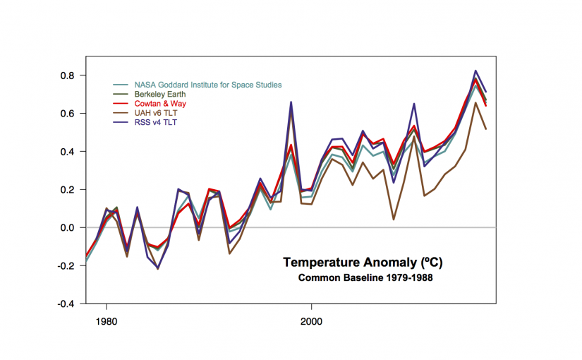
Figure 1. Test of the Hasselmann model through a regression analysis, where the coloured curves are the best-fit modelled values for Q based on the Hasselmann model and global mean temperatures (PDF).
It is clear that the model fails for the dips in the forcing connected volcanic eruptions (Figure 1). We also see a substantial scatter in both  (some values are even negative and hence unphysical) and
  (Figure 2).

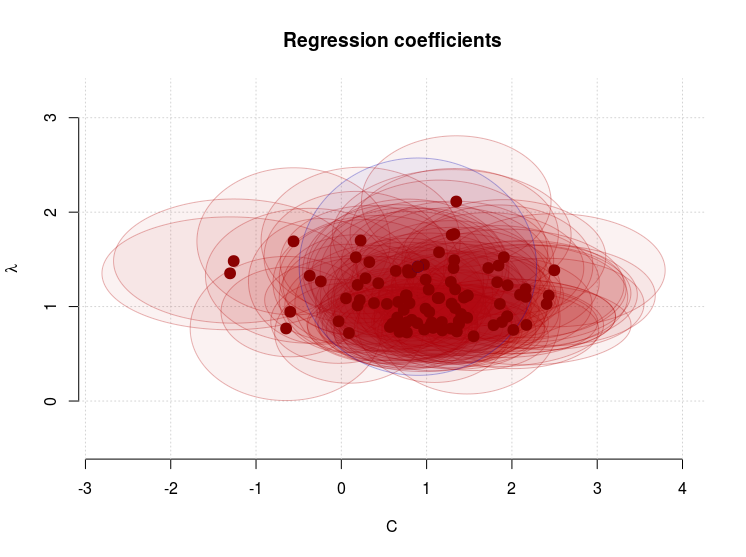
Figure 2. The regression coefficients. Negative values for C are unphysical and suggest that the Hasselmann model is far from perfect. The estimated error margins for C are substantial, however, and also include positive values. Blue point shows the estimates for NCEP/NCAR reanalysis. The shaded areas cover the best estimates plus/minus two standard errors (PDF).
The climate sensitivity is closest associated with , for which the mean estimate was 1.11 , with a 5-95-percentile interval of 0.74-1.62.
We can use these estimates in a naive attempt to calculate the temperature response for a stable climate with  and a doubled forcing associated with increased CO2.
It’s plain mathematics. I took a doubling of 1998 CO2-forcing of 2.43 from Crowley (2000), and used the non-zero terms in the Hasselmann model,
  .
.
The mean temperature response to a doubled CO2-forcing for GCMs was 2.36 , with a 90% confidence interval: 1.5 – 3.3
 . The estimate from reanalysis was 1.71
The true equilibrium climate sensitivity for the climate models used in this demonstration is in the range 2.1 – 4.4 , and the transient climate sensitivity is 1.2 – 2.6 (IPCC AR5, Table 8.2).
This demonstration suggests that the Hasselmann model underestimates the climate sensitivity and the over-simplified framework on which it is based precludes high precision.
Another assumption made in the calculations was that the climate forcing Q looks like a white noise after the removal of the long-term trends.
This too is questionable, as there are reasons to think the ocean uptake of heat varies at different time scales and may be influenced by ENSO, the Pacific Decadal Oscillation (PDO), and the Atlantic Multi-decadal Oscillation (AMO). The solar irradiance also has an 11-year cycle component and volcanic eruptions introduce spikes in the forcing (see Figure 1).
Cox et al.’s calculations were also based on another assumption somewhat related to different time scales for different feedback mechanisms: a constant “heat capacity” represented by C in the equation above.
The real-world “heat capacity” is probably not constant, but I would expect it to change with temperature.
Since it reflects the capacity of the climate system to absorb heat, it may be influenced by the planetary albedo (sea-ice and snow) and ice-caps, which respond to temperature changes.
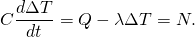
It’s more likely that C is a non-linear function of temperature, and in this case, the equation describing the Hasselmann model would look like:
(2) 
Cox et al.’s calculations of the equilibrium climate sensitivity used a key metric  which was derived from the Hasselmann model and assumed a constant C:
  . This key metric would be different if the heat capacity varied with temperature, which subsequently would affect the end-results.
I also have an issue with the confidence interval presented for the calculations, which was based on one standard deviation  . The interval of
  represents a 66% probability, and can be illustrated with three numbers: and two of them are “correct” and one “wrong”, which means there is a 1/3 chance that I pick the “wrong” number if I were to randomly pick one of the three.
To be fair, the study also stated the 90% confidence interval, but it was not emphasised in the abstract nor in the press-coverage.
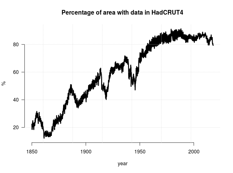
One thing that was not clear, was whether the analysis, that involved both observed temperatures from the HadCRUT4 dataset and global climate models, took into account the fact that the observations do not cover 100% of Earth’s surface (see RC post ‘Mind the Gap!’).
A spatial mask would be appropriate to ensure that the climate model simulations provide data for only those regions where observations exists. Moreover, it would have to change over time because the thermometer observations have covered a larger fraction of Earth’s area with time (see Figure 3).
An increase in data coverage will affect the estimated variance  and one-year autocorrelation
  associated with the global mean temperature, which also should influence the the metric .

Figure 3. The area of Earth’s surface with valid temperature data (PDF).
My last issue with the calculations is that the traditional definition of climate sensitivity only takes into account changes in the temperature. However, there is also a possibility that a climate change involves a change in the hydrological cycle. I have explained this possibility in a review of the greenhouse effect (Benestad, 2017), and this possibility would add another term the equation describing the Hasselmann model.
I nevertheless think the study is interesting and it is impressive that the results are so similar to previously published results. However, I do not think the results are associated with the stated precision because of the assumptions and the simplifications involved. Hence, I disagree with the following statement presented in the Guardian:
These scientists have produced a more accurate estimate of how the planet will respond to increasing CO2 levels
References
P.M. Cox, C. Huntingford, and M.S. Williamson, “Emergent constraint on equilibrium climate sensitivity from global temperature variability”, Nature, vol. 553, pp. 319-322, 2018. http://dx.doi.org/10.1038/nature25450
T.J. Crowley, “Causes of Climate Change Over the Past 1000 Years”, Science, vol. 289, pp. 270-277, 2000. http://dx.doi.org/10.1126/science.289.5477.270
R.E. Benestad, “A mental picture of the greenhouse effect”, Theoretical and Applied Climatology, vol. 128, pp. 679-688, 2016. http://dx.doi.org/10.1007/s00704-016-1732-y