Rocky mountain lodgepole Pine (Pinus contorta var. latifolia)

American Forests National Tree Register, Species: Rocky mountain lodgepole Pine (Pinus contorta var. latifolia), State: OR
Description OR ID #231

Location Grant County, OR

Rocky Mountain lodgepole PINE

Pinus contorta var. latifolia

This champion Rocky Mountain lodgepole Pine of Oregon made its debut on the list of American Forests Champion Trees in 2017, as it is the largest known tree of its species in the country. By recognizing these champions, we recognize the beauty and critical ecosystem services provided by our biggest and oldest trees.

jQuery(document).ready(function(){
jQuery(‘.bt_images_slider’).bxSlider({
mode: ‘fade’,
captions: false,
adaptiveHeight: true,
slideWidth: ‘auto’,
preloadImages: ‘all’,
pager: false,
controls: false,
nextSelector: ‘#bt_images_slider’,
auto: false,
speed: 0
});
});

STATUS Champion
Tree circumference 136
height 110
crown spread 44
Total points 257

LOCATION Grant County, OR
Nominated by Scott McDonald
Year Nominated 2000
Date crowned 2017-08-15

Other Champion Trees

Pinus attenuata

Pinus ponderosa var. ponderosa

Pinus sabiniana

Help us protect ecosystems where Big Trees thrive

Ways to Engage

search-icon

Search

Search the American Forests Champion Tree national register.

Nominate

Nominate a big tree that you think can achieve champion status.

Explore

Browse stories on our blog, Loose Leaf, and get to know the people and champions that make up the program.

Subscribe

Sign up for our big tree email list and receive year-round updates on the program.

The post Rocky mountain lodgepole Pine (Pinus contorta var. latifolia) appeared first on American Forests.

White Ash (Fraxinus americana)

American Forests National Tree Register, Species: White Ash (Fraxinus americana), State: NY
Description Lou Sebest 845-831-8780 ext. 316 can confirm measurements already shown on NYS registration and measurement information at: http://www.dec.ny.gov/docs/lands_forests_pdf/treechamp0909com.pdf

James Castagna resubmitted tree to save White ash from future destruction. Original nominator still stands.

Location Rockland, NY

White ASH

Fraxinus americana

This champion White Ash of New York made its debut on the list of American Forests Champion Trees in 2017, as it is the largest known tree of its species in the country. By recognizing these champions, we recognize the beauty and critical ecosystem services provided by our biggest and oldest trees.

jQuery(document).ready(function(){
jQuery(‘.bt_images_slider’).bxSlider({
mode: ‘fade’,
captions: false,
adaptiveHeight: true,
slideWidth: ‘auto’,
preloadImages: ‘all’,
pager: false,
controls: false,
nextSelector: ‘#bt_images_slider’,
auto: false,
speed: 0
});
});

STATUS Champion
Tree circumference 283
height 84
crown spread 84
Total points 388

LOCATION Rockland, NY
Nominated by F. Arthur Belcher
Year Nominated 1983
Date crowned 2017-08-16

Other Champion Trees

Fraxinus americana

Fraxinus americana

Fraxinus texensis

Help us protect ecosystems where Big Trees thrive

Ways to Engage

search-icon

Search

Search the American Forests Champion Tree national register.

Nominate

Nominate a big tree that you think can achieve champion status.

Explore

Browse stories on our blog, Loose Leaf, and get to know the people and champions that make up the program.

Subscribe

Sign up for our big tree email list and receive year-round updates on the program.

The post White Ash (Fraxinus americana) appeared first on American Forests.

Pecan (Carya illinoinensis)

American Forests National Tree Register, Species: Pecan (Carya illinoinensis), State: VA
Description all i said to people that you have have to see the tree .
you can go to www.cnr.vt.edu/4H/BIGTREE/bigtree_detail.cfm?AutofieldforPrimaryKey=982 you can see a picture of my tree

8/15/17 updated status from dethroned to co-champion. Larger tree that dethroned this tree has since been dethroned due to the 10-year rule. Justin Hynicka

Location isle of wight, VA

PECAN

Carya illinoinensis

This champion Pecan of Virginia made its debut on the list of American Forests Champion Trees in 2014, as it is the largest known tree of its species in the country. By recognizing these champions, we recognize the beauty and critical ecosystem services provided by our biggest and oldest trees.

jQuery(document).ready(function(){
jQuery(‘.bt_images_slider’).bxSlider({
mode: ‘fade’,
captions: false,
adaptiveHeight: true,
slideWidth: ‘auto’,
preloadImages: ‘all’,
pager: false,
controls: false,
nextSelector: ‘#bt_images_slider’,
auto: false,
speed: 0
});
});

STATUS Champion
Tree circumference 274
height 106
crown spread 92
Total points 403

LOCATION isle of wight, VA
Nominated by Ernest J.W. Goodrich
Year Nominated 2009
Date crowned 2014-04-14

Other Champion Trees

Carya illinoinensis

Maclura pomifera

Styrax americanus

Help us protect ecosystems where Big Trees thrive

Ways to Engage

search-icon

Search

Search the American Forests Champion Tree national register.

Nominate

Nominate a big tree that you think can achieve champion status.

Explore

Browse stories on our blog, Loose Leaf, and get to know the people and champions that make up the program.

Subscribe

Sign up for our big tree email list and receive year-round updates on the program.

The post Pecan (Carya illinoinensis) appeared first on American Forests.

Buttonmangrove (Conocarpus erectus)

American Forests National Tree Register, Species: Button-mangrove (Conocarpus erectus), State: FL
Description Circ. Ht measured above root on NE side.

Location Palm Beach, FL

BUTTON-MANGROVE

Conocarpus erectus

This champion Button-mangrove of Florida made its debut on the list of American Forests Champion Trees in 2017, as it is the largest known tree of its species in the country. By recognizing these champions, we recognize the beauty and critical ecosystem services provided by our biggest and oldest trees.

jQuery(document).ready(function(){
jQuery(‘.bt_images_slider’).bxSlider({
mode: ‘fade’,
captions: false,
adaptiveHeight: true,
slideWidth: ‘auto’,
preloadImages: ‘all’,
pager: false,
controls: false,
nextSelector: ‘#bt_images_slider’,
auto: false,
speed: 0
});
});

STATUS Champion
Tree circumference 201
height 44
crown spread 73
Total points 263

LOCATION Palm Beach, FL
Nominated by Kenneth Van der Hulse & Donald L. Lockha
Year Nominated 1974
Date crowned 2017-08-15

Other Champion Trees

Conocarpus erectus

Pithecellobium keyense

Acoelorraphe wrightii

Help us protect ecosystems where Big Trees thrive

Ways to Engage

search-icon

Search

Search the American Forests Champion Tree national register.

Nominate

Nominate a big tree that you think can achieve champion status.

Explore

Browse stories on our blog, Loose Leaf, and get to know the people and champions that make up the program.

Subscribe

Sign up for our big tree email list and receive year-round updates on the program.

The post Buttonmangrove (Conocarpus erectus) appeared first on American Forests.

White Mulberry (Morus alba)

American Forests National Tree Register, Species: White Mulberry (Morus alba), State: OH
Description Tree has some structural problems and hollowing out

8/15/17 – previous champion was damaged elevating this and two other trees to co-champions. Justin Hynicka

Location Sandusky County, OH

White MULBERRY

Morus alba

This champion White Mulberry of Ohio made its debut on the list of American Forests Champion Trees in 2014, as it is the largest known tree of its species in the country. By recognizing these champions, we recognize the beauty and critical ecosystem services provided by our biggest and oldest trees.

jQuery(document).ready(function(){
jQuery(‘.bt_images_slider’).bxSlider({
mode: ‘fade’,
captions: false,
adaptiveHeight: true,
slideWidth: ‘auto’,
preloadImages: ‘all’,
pager: false,
controls: false,
nextSelector: ‘#bt_images_slider’,
auto: false,
speed: 0
});
});

STATUS Champion
Tree circumference 261
height 54
crown spread 58
Total points 330

LOCATION Sandusky County, OH
Nominated by Carl J. Dymond
Year Nominated 1965
Date crowned 2014-04-16

Other Champion Trees

Morus alba

Morus alba

Morus nigra

Help us protect ecosystems where Big Trees thrive

Ways to Engage

search-icon

Search

Search the American Forests Champion Tree national register.

Nominate

Nominate a big tree that you think can achieve champion status.

Explore

Browse stories on our blog, Loose Leaf, and get to know the people and champions that make up the program.

Subscribe

Sign up for our big tree email list and receive year-round updates on the program.

The post White Mulberry (Morus alba) appeared first on American Forests.

Bitternut Hickory (Carya cordiformis)

American Forests National Tree Register, Species: Bitternut Hickory (Carya cordiformis), State: MD
Description Tree has multiple leaders above 8′. Tree has been cleaned of grapevine, but shows some minor damage from vines.

8/15/17 status restored to co-champ as larger tree that dethroned this tree was determined to be ineligible due to multiple leaders. Justin Hynicka

Location Harford, MD

Bitternut HICKORY

Carya cordiformis

This champion Bitternut Hickory of Maryland made its debut on the list of American Forests Champion Trees in 2017, as it is the largest known tree of its species in the country. By recognizing these champions, we recognize the beauty and critical ecosystem services provided by our biggest and oldest trees.

jQuery(document).ready(function(){
jQuery(‘.bt_images_slider’).bxSlider({
mode: ‘fade’,
captions: false,
adaptiveHeight: true,
slideWidth: ‘auto’,
preloadImages: ‘all’,
pager: false,
controls: false,
nextSelector: ‘#bt_images_slider’,
auto: false,
speed: 0
});
});

STATUS Champion
Tree circumference 198
height 108
crown spread 103
Total points 332

LOCATION Harford, MD
Nominated by Harford County Government
Year Nominated 2009
Date crowned 2017-08-15

Other Champion Trees

Carya cordiformis

Carya tomentosa

Help us protect ecosystems where Big Trees thrive

Ways to Engage

search-icon

Search

Search the American Forests Champion Tree national register.

Nominate

Nominate a big tree that you think can achieve champion status.

Explore

Browse stories on our blog, Loose Leaf, and get to know the people and champions that make up the program.

Subscribe

Sign up for our big tree email list and receive year-round updates on the program.

The post Bitternut Hickory (Carya cordiformis) appeared first on American Forests.

Live in a City? Bring Nature to You

August 16th, 2017|Tags: , |0 Comments

.fusion-fullwidth-1 {
padding-left: px !important;
padding-right: px !important;
}

By Allie Wisniewski, American Forests

When you call a bustling city home, it can often be tough to connect with nature. Don’t give up hope, though – there are plenty of ways to bring nature to you.

Spend Time in Local Parks

The only thing they need now is a chessboard! Credit: Miki Yoshihito

If you live in a city, pure, unadulterated nature can be hard to come by. Thankfully, urban parks exist, and with their abundance of trees, grass, shrubs and wildflowers, they can get pretty close to wilderness. A study by researchers at the University of Illinois found that “viewing tree canopy in communities can significantly aid stress recovery.” Browsing this list of the best urban parks in the country should assure you that there’s always greenspace close by waiting to provide you with that much-needed serenity.

Read Nature-Themed Books

You’ll need a few more than he has to really connect with nature, but this is a good start. Credit: Steven Guzzardi

Okay, sure, it’s not exactly the same thing, but never underestimate the power of imagery to transport you far beyond the confines of your bedroom. If reading in a forest isn’t feasible for you, at least you can read about a forest. Refer to this list if you’re searching for that perfect mental getaway — Goodreads has catalogued 546 of the best nature-themed books out there. If that isn’t a thorough compilation, I don’t know what is. From Thoreau’s classic “Walden” to Bill Bryson’s more contemporary “A Walk in the Woods”, you’re sure to find a tale that will help simulate the outdoor adventure you’re craving.

Plant an Indoor Garden

An indoor garden also has the side-effect of impressing your guests with your ability to sustain life! Credit: Ella Schierbeck

One of the best ways to connect to nature is to get up close and personal — to really get your hands dirty and grow your own food and flowers. Backyards aren’t exactly conventional, though, when it comes to urban housing, so traditional gardening might prove a bit tricky for those of you city-dwellers with limited space. With a little creativity and determination, however, anything is possible. Even if you consider yourself a “brown thumb,” growing potted herbs and flowers on your balcony or windowsill is an easily attainable feat. To get started, check out these low-maintenance plants for your indoor garden.

Listen to Nature Sounds

Finding zen within the city could be as easy as closing your eyes and putting on your headphones. Credit: Tina Leggio

If you can’t access the outdoors, you can always bring the outdoors in. Thanks to streaming apps like Spotify that offer dozens of nature playlists, it’s never been easier to access the sounds of wilderness. YouTube is another great resource for nature soundtracks, and some of my favorite apps include Naturespace and Ambiance. When your urban home is finally filled with house plants, your own indoor garden and scattered piles of nature-themed books, the sweet calls of songbirds in the background is just what you need to round off the ambiance.

The post Live in a City? Bring Nature to You appeared first on American Forests.

Sensible Questions on Climate Sensitivity

Guest Commentary by Cristian Proistosescu, Peter Huybers and Kyle Armour

tl;dr 

Two recent papers help bridge a seeming gap between estimates of climate sensitivity from models and from observations of the global energy budget. Recognizing that equilibrium climate sensitivity cannot be directly observed because Earth’s energy balance is a long way from equilibrium, the studies instead focus on what can be inferred about climate sensitivity from historical trends. Calculating a climate sensitivity from the simulations that is directly comparable with that observed shows both are consistent. Crucial questions remain, however, regarding how climate sensitivity will evolve in the future.

Background

The recent papers, by Kyle Armour (hereafter A17) and by us (Proistosescu and Huybers, 2017) (hereafter PH17), build on a large literature documenting the time-dependence of climate feedbacks in models. They make quantitative apples-to-apples comparisons between the climate sensitivities simulated by CMIP5 models and those inferred from global energy budget observations.

[Aside: For brevity, we refer to the global energy budget constraints as “observations”. In reality, these constraints are not purely observational; they combine surface and ocean temperature observations over the recent transient evolution of the climate system with model-based estimates of historical radiative forcing and of the global energy imbalance during early-industrial climate. Further, inference of climate sensitivity from these observations rely upon a physical model that entails some strong simplifications.]

Because feedbacks may change over time as patterns of warming evolve, observations made today do not necessarily provide estimates of the long-term, equilibrium climate sensitivity (ECS). Rather, they constrain a quantity that we call the inferred (A17), or instantaneous (PH17), climate sensitivity (ICS). The two studies were performed independently using distinct methodologies, and both find that ICS values are systematically lower than ECS values within CMIP5 models. Moreover, they find that model-derived ICS values are consistent with ICS values inferred from observations.


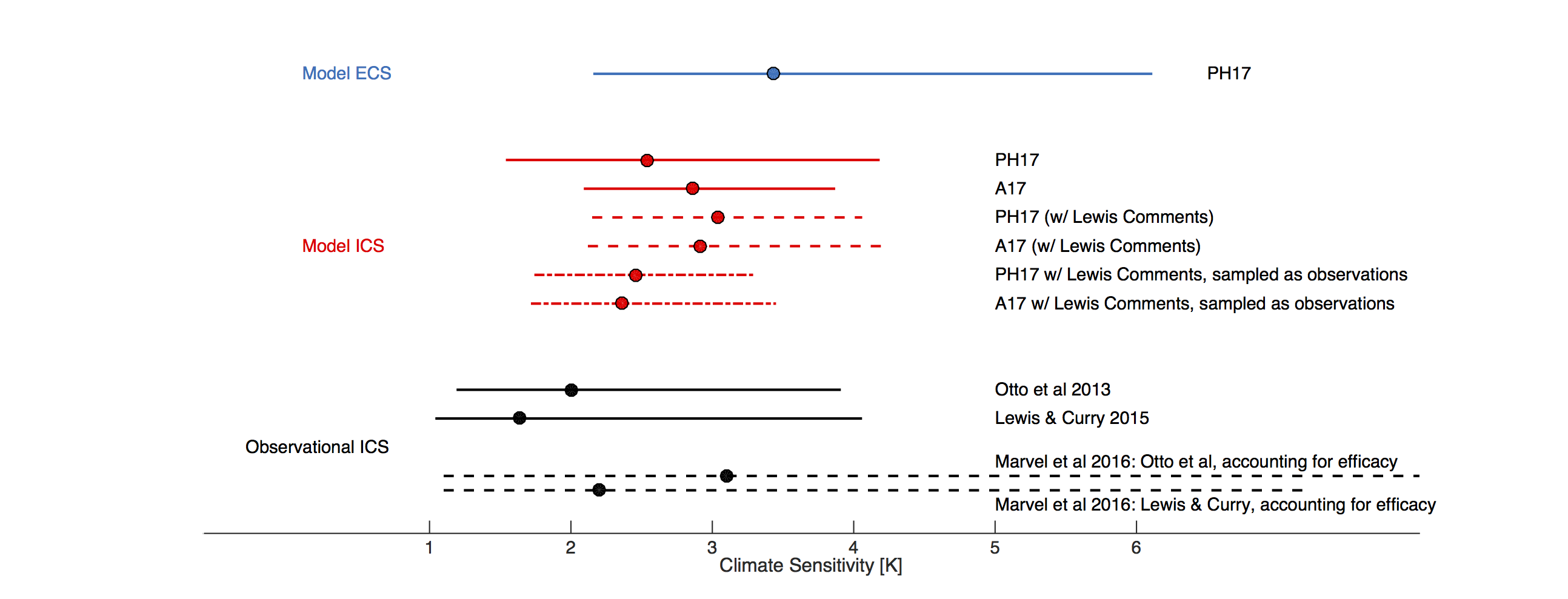
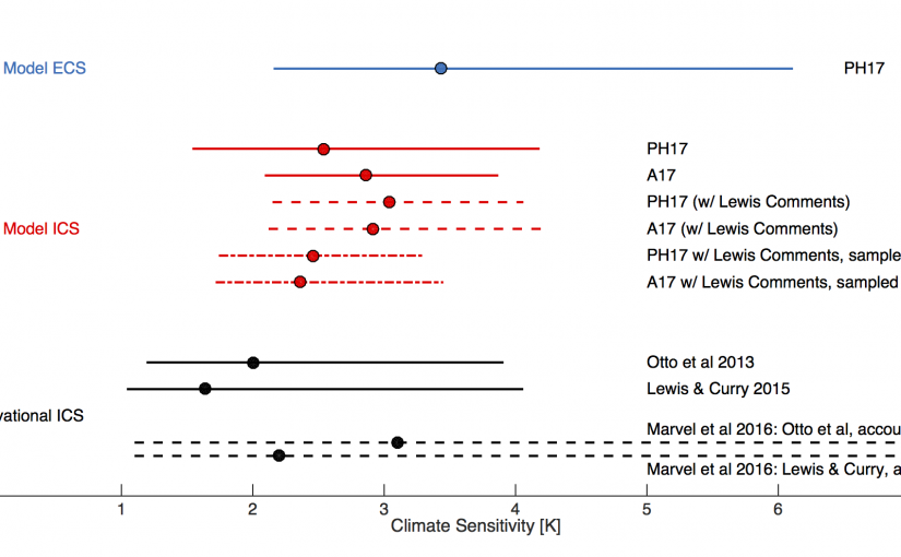
Figure shows model Equilibrium Climate Sensitivity (ECS, blue, from PH17), compared with observationally- and model-derived Inferred/Instantaneous Climate Sensitivity (ICS, black and red). Circles denote medians, while the line denotes the 5-95% confidence interval. Solid lines indicate published estimates, dashed lines indicate PH17 and A17 values with Nic Lewis’ comments taken into account, and dot-dashed lines indicate PH17 and A17 values with both the Lewis correction and the Richardson et al (2015) correction.

Of mountains and molehills

Nic Lewis has posted some criticisms of both papers (A17 critique, PH17 critique) where he proposes changes to these studies that supposedly render the models and data again in disagreement. The criticisms focus on the treatment of radiative forcing within the models which is used in the calculation of ICS values. We approach these criticisms by exploring their implications for the resulting ICS estimates, without necessarily implying agreement.

For A17, Lewis suggests that one should (i) assume that CO2 forcing increases slightly faster than logarithmically with CO2 concentration, rather than linearly, as is traditional[1], and (ii) estimate model CO2 forcing values by a different method[2]. Accounting for these two effects increases model-mean and median ICS by ~0.1°C. For PH17 the suggestions are to (i) adjust historical forcing to account for the average pre-industrial volcanic forcing[3], (ii) rescale the radiative forcing associated with a CO2 doubling for each model when calculating ICS[4], and (iii) better account for the difference between instantaneous and effective radiative forcing, a point that was raised in PH17. While the last suggested adjustment almost certainly conflates time-dependence of feedbacks with stratospheric and tropospheric adjustment, we nonetheless explore the impact of adding Lewis’ upward correction of 0.1°C.


[1]A17 employed the standard assumption that CO2 forcing increases linearly with the logarithm of concentration, while recent work suggests that CO2 forcing might increase slightly faster than linearly. Assuming this forcing nonlinearity decreases model ICS by 0.04°C, on average.

[2]A17 estimated CO2 forcing using linear regression of global radiative imbalance on global temperature over years 1-5 of each model’s abrupt CO2 quadrupling simulations. This choice was made to avoid forcing estimates being biased by the nonlinear relationship between radiative imbalance and temperature that typically emerges beyond year 5. Using years 1-20 for this calculation, as Lewis suggests, seems unwise to us. But doing so increases model ICS by 0.09°C, on average. A third suggestion was to include additional CMIP5 models in the analysis; while we do not do so here, we estimate that including them would bring model-mean ICS back to near the A17 value since most of the additional models are variants of those already included that happen to have low ICS.

[3]Temperature change is considered as an anomaly with respect to pre-industrial climate. Thus, volcanic forcing should also be considered as anomalies with respect to the average pre-industrial forcing. The issues of pre-industrial volcanic forcing can be largely avoided by considering the same averaging interval as in Lewis and Curry (2015), raising model ICS by an average of 0.1°C.

[4]Radiative forcing PH17 inferred from the CMIP5 models (which averages 3.9 W/m2) is larger for a doubling of CO2 than the estimate generally used elsewhere, including in Lewis’s estimates (3.7 W/m2, ref. AR5 TS & 9.7.1, which relies on a subset of the CMIP5 models). In order to make results comparable, PH17 rescaled radiative forcing to the commonly-used AR5 value.

In the figure, we show both the original A17 and PH17 estimates of model ICS, and versions that take into account Lewis’s suggestions. The most notable change is that the PH17 model-median ICS estimate increases from 2.5 to 3.0°C, while the 5-95% credible interval narrows from 1.6 to 4.2°C to a range of 2.2 to 4.0°C. This shift is primarily in response to rescaling radiative forcing using model specific values, and it leads to better agreement between the median values of PH17 and A17. However, regardless of the methodology used, or whether or not Lewis’ suggestions are accounted for, the core results still hold: model values of ICS are consistent with observational ICS values.

Should we be concerned by the remaining offset?

Although consistent, the ranges of historical and model based ICS values do not completely overlap. However, there are additional effects that could be taken into account that would make the estimates more congruent. When sampled in a manner consistent with observations, by accounting for spatial coverage and differences between sea-surface and near-surface-air temperatures, changes in model temperature over the historical period are reduced by a median of 19% (i.e. Richardson et al (2015)). A proportional correction to model ICS is illustrated in the figure. Additionally, there is significant uncertainty in the magnitude and efficacy of non-CO2 forcing agents. There is enough uncertainty in fact, that accounting for the efficacy can broaden the range of observational ICS to easily contain all model estimates (Figure 1).

Furthermore, while model-median ICS is based on the forced response in a model ensemble, the observational ICS depends on a single realization of Earth’s warming, the details of which are sensitive to the phase of natural variability affecting the pattern of surface warming over the periods considered. Thus, the observed estimate of ICS is almost certainly perturbed from its expected value (i.e., what would be obtained from perfect knowledge of an infinite ensemble of Earth histories). Recent evidence suggests that observed temperature patterns in recent decades, associated with a cooling of the East Pacific, can lead to a more negative cloud feedback than that seen in the historical response in models over the same period. It seems important to determine whether the inability of models to simulate these recent patterns is indicative of model deficiencies or simply a consequence of natural variability.

Since both estimates have differing sources of uncertainty, demanding agreement between the best-estimate historical ICS and best-estimate model ICS would constitute over-fitting. Additionally, given the fact that the model ensemble is an ensemble of opportunity, we don’t expect the model range to cover the full uncertainty range. Still, it is worth considering the lack of model coverage in the range of low ICS. This discrepancy may reflect that while low values of ICS are allowed by observational constraints (associated with a low aerosol forcing), it is challenging to construct climate models that produce such low ICS values, as it requires a more-negative cloud feedback that is difficult to reconcile with current mechanistic understandings. Better constraints on historical aerosol forcing and forcing efficacy might go a long way towards understanding the plausibility of low ICS values (e.g. Marvel et al, 2016).

What is the magnitude of ECS? (hint:≠ICS)

An important core finding of A17 and PH17 is that values of ICS drawn from the historical record are not sufficient to constrain values of ECS. Indeed, within models, ICS and ECS differ as the strength of radiative feedbacks change over time as patterns of surface temperature evolve with warming. PH17 demonstrated that portions of the climate system that respond over centennial timescales (such as the southern oceans) are important amplifiers of climate sensitivity in the models – a slow-mode response leading to values of ECS that are higher than the values of ICS that reflect more transient warming. Increasing sensitivity over time seems to be associated with a low-cloud feedback excited by warming in the Eastern Equatorial Pacific and Southern Ocean. This slow-mode response (and thus ECS) is essentially unconstrained by global energy budget observations because warming in these regions has been small, possibly held back by upwelling water from the ocean interior.

Key research targets should be improving understanding of (i) how the east-west temperature gradient in the Pacific Ocean will evolve in the future, and (ii) how low-level cloud (and other) feedbacks will respond, in turn. Zhou et al (2017) suggest that feedbacks can vary with the surface warming pattern, at least on decadal timescales. Yet, it is not known whether the magnitude by which feedbacks evolve within the models is realistic. A major challenge going forward is to develop instrumental observations capable of constraining these processes. Another potential path to better understanding slow-mode contributions to ECS is to explore paleoclimate changes occurring over timescale where the climate has had more time to fully come into equilibrium (e.g., PALAEOSENS).

As usual, it will be the interplay between theoretical exploration and observational analysis that will build our understanding of climate sensitivity. Lewis’ comments have helped to sharpen consideration of the topic, but we need not make mountains of difference out of molehills. Model ICS estimates strongly overlap with observed ICS uncertainty ranges, and proposed alterations involve only small modifications. More interesting at this point is to explore how future warming could diverge from historical patterns, and how climate feedbacks in the future might be different from those at present.


Acknowledgements

We thank Nic Lewis and Gavin Schmidt for comments on a draft of this post. We want to note that on the basis of as-of-yet unpublished research, Nic disagrees with our use of the Kummer and Dessler upward correction of observational ICS due to aerosol efficacy.

References


  1. K.C. Armour, “Energy budget constraints on climate sensitivity in light of inconstant climate feedbacks”, Nature Climate Change, vol. 7, pp. 331-335, 2017. http://dx.doi.org/10.1038/nclimate3278


  2. C. Proistosescu, and P.J. Huybers, “Slow climate mode reconciles historical and model-based estimates of climate sensitivity”, Science Advances, vol. 3, pp. e1602821, 2017. http://dx.doi.org/10.1126/sciadv.1602821


  3. C.A. Senior, and J.F.B. Mitchell, “The time-dependence of climate sensitivity”, Geophysical Research Letters, vol. 27, pp. 2685-2688, 2000. http://dx.doi.org/10.1029/2000gl011373


  4. T. Andrews, J.M. Gregory, and M.J. Webb, “The Dependence of Radiative Forcing and Feedback on Evolving Patterns of Surface Temperature Change in Climate Models”, Journal of Climate, vol. 28, pp. 1630-1648, 2015. http://dx.doi.org/10.1175/jcli-d-14-00545.1


  5. P.M. Forster, “Inference of Climate Sensitivity from Analysis of Earth’s Energy Budget”, Annual Review of Earth and Planetary Sciences, vol. 44, pp. 85-106, 2016. http://dx.doi.org/10.1146/annurev-earth-060614-105156


  6. M. Richardson, K. Cowtan, E. Hawkins, and M.B. Stolpe, “Reconciled climate response estimates from climate models and the energy budget of Earth”, Nature Climate Change, vol. 6, pp. 931-935, 2016. http://dx.doi.org/10.1038/nclimate3066


  7. G. Myhre, E.J. Highwood, K.P. Shine, and F. Stordal, “New estimates of radiative forcing due to well mixed greenhouse gases”, Geophysical Research Letters, vol. 25, pp. 2715-2718, 1998. http://dx.doi.org/10.1029/98gl01908


  8. B. Byrne, and C. Goldblatt, “Radiative forcing at high concentrations of well-mixed greenhouse gases”, Geophysical Research Letters, vol. 41, pp. 152-160, 2014. http://dx.doi.org/10.1002/2013gl058456


  9. N. Lewis, and J.A. Curry, “The implications for climate sensitivity of AR5 forcing and heat uptake estimates”, Climate Dynamics, vol. 45, pp. 1009-1023, 2014. http://dx.doi.org/10.1007/s00382-014-2342-y


  10. J.R. Kummer, and A.E. Dessler, “The impact of forcing efficacy on the equilibrium climate sensitivity”, Geophysical Research Letters, vol. 41, pp. 3565-3568, 2014. http://dx.doi.org/10.1002/2014gl060046


  11. K. Marvel, G.A. Schmidt, R.L. Miller, and L.S. Nazarenko, “Implications for climate sensitivity from the response to individual forcings”, Nature Climate Change, vol. 6, pp. 386-389, 2015. http://dx.doi.org/10.1038/nclimate2888


  12. C. Zhou, M.D. Zelinka, and S.A. Klein, “Impact of decadal cloud variations on the Earth’s energy budget”, Nature Geoscience, vol. 9, pp. 871-874, 2016. http://dx.doi.org/10.1038/ngeo2828


  13. R. Knutti, R. Furrer, C. Tebaldi, J. Cermak, and G.A. Meehl, “Challenges in Combining Projections from Multiple Climate Models”, Journal of Climate, vol. 23, pp. 2739-2758, 2010. http://dx.doi.org/10.1175/2009jcli3361.1


  14. J.R. Kummer, and A.E. Dessler, “The impact of forcing efficacy on the equilibrium climate sensitivity”, Geophysical Research Letters, vol. 41, pp. 3565-3568, 2014. http://dx.doi.org/10.1002/2014GL060046


  15. K.C. Armour, J. Marshall, J.R. Scott, A. Donohoe, and E.R. Newsom, “Southern Ocean warming delayed by circumpolar upwelling and equatorward transport”, Nature Geoscience, vol. 9, pp. 549-554, 2016. http://dx.doi.org/10.1038/ngeo2731


  16. E.J. Rohling, E.J. Rohling, A. Sluijs, H.A. Dijkstra, P. Köhler, R.S.W. van de Wal, A.S. von der Heydt, D.J. Beerling, A. Berger, P.K. Bijl, M. Crucifix, R. DeConto, S.S. Drijfhout, A. Fedorov, G.L. Foster, A. Ganopolski, J. Hansen, B. Hönisch, H. Hooghiemstra, M. Huber, P. Huybers, R. Knutti, D.W. Lea, L.J. Lourens, D. Lunt, V. Masson-Demotte, M. Medina-Elizalde, B. Otto-Bliesner, M. Pagani, H. Pälike, H. Renssen, D.L. Royer, M. Siddall, P. Valdes, J.C. Zachos, and R.E. Zeebe, “Making sense of palaeoclimate sensitivity”, Nature, vol. 491, pp. 683-691, 2012. http://dx.doi.org/10.1038/nature11574

Byproducts of Bees

August 15th, 2017|0 Comments

.fusion-fullwidth-2 {
padding-left: px !important;
padding-right: px !important;
}

By Melanie Friedel, American Forests

Credit: Jim Bauer

You probably know bees as the insects that pollinate flowers or the pests that sting your cousin and ruin your family barbecues every summer, but you might be surprised to hear that they’re not the only things that bees do!

Yes, we need bees to pollinate flowers so that we can grow crops and maintain habitats and food sources for animals and insects. This also helps ensure that plants can be around to provide oxygen, making the world a better place. But it’s rare that we give bees the credit they deserve for providing us with products we use every day.

Honey, of course, is a big one. Bees make honey by collecting nectar from flower blossoms, bringing it back to the hive, chewing it, passing it to other bees who continue to chew it and eventually depositing it into honeycomb once it’s thick enough. While the honey is stored in the honeycomb cell, the bees fan it with their wings until it dries out and becomes stickier. Eventually it reaches our kitchens, sometimes still in the honeycomb! We use it as a natural sweetener in food and drinks, but it also eases sore throats, boosts our immune systems — especially our immunity to local allergens if we eat local honey — and is both an antioxidant and anti-inflammatory. Who knew?

A less common bee byproduct you should know about is propolis. Bees make it by combining sap from plants and trees with beeswax. Different types of plants and trees result in different types of propolis, so bees in different places make varying kinds. Bees use propolis to build their hives, while we use it for medicine. Propolis contains more than 300 compounds, most of which are antioxidants and immune-system boosters. You can find it at pharmacies or health food stores, ranging from liquid sprays for a sore throat to hard candies for a healthy treat. Its many benefits include antibacterial, antiviral, antifungal and anti-inflammatory powers. Use it on your throat, a cut, a swollen ankle, on your skin to soften it and reduce redness, or throw some into your morning coffee or juice!

Most honey bees eat honey, but the queen bee gets something much more prestigious: royal jelly. And we can use it too. Young female worker bees combine pollen with the materials in their glands to produce the jelly, which is full of nutrients and minerals including calcium, iron, potassium and an array of amino acids. Its list of benefits seems endless. Like honey and propolis, it boosts our immune systems and fights seasonal allergies, but it also supports our kidney, pancreas and liver, reduces cholesterol, works as a probiotic supporting all-around health, makes our skin softer, can help heal wounds, prevents Alzheimer’s disease, and might even help with diabetes.

The power of these products is astounding and certainly worth recognizing. We can thank bees for much more than the beautiful flowers they allow us to enjoy, and with all of these benefits, we might even be able to forgive them for the occasional sting. Next time you’re at your local market, give these bee byproducts a shot — you might just find out that nature produces the best medicine of all.

The post Byproducts of Bees appeared first on American Forests.

The Best Hiking Trails to Spot Wildlife

August 14th, 2017|Tags: , |0 Comments

.fusion-fullwidth-1 {
padding-left: px !important;
padding-right: px !important;
}

By Allie Wisniewski, American Forests

Hidden Lake Overlook, Glacier National Park

Glacier National Park in Montana is home to nearly 70 species of mammals, so although it’s never all that difficult to spot its resident fauna, the Hidden Lake Overlook trail is particularly well known for frequent wildlife sightings. At only 1.35 miles, this trail is especially great for those who aren’t looking for a strenuous journey.

What you’ll see: Bighorn sheep, mountain goats, marmots, wolverines

Cades Cove, Great Smoky Mountains National Park

While Cades Cove is one of the park’s most popular destinations, opportunities for viewing wildlife remain abundant. The valley is surrounded by mountains and an 11-mile loop encircles the cove. While the road can also be driven, it’s closed to motor vehicles until 10:00 a.m. every Saturday and Wednesday for the enjoyment of wildlife-seeking hikers and bikers.

What you’ll see: White-tailed deer, black bears, elk, coyotes, turkeys, groundhogs, skunks, raccoons

Trail Ridge Road, Rocky Mountain National Park

For avid bird-watchers, Trail Ridge Road is way to go. Known for its alpine tundra terrain, this trail is ideal for spotting marmots and pikas (small, light-colored mammals) as well as a variety of birds, though some are rare and generally difficult to spot. White-tailed ptarmigans, for example, are some of the most sought-after birds in the park. Are you up for the challenge?

What you’ll see: Clark’s nutcrackers, Steller’s jays, golden eagles, prairie falcons, marmots, pikas

Rialto Beach, Olympic National Park

Between April and May and again in October and November, Rialto Beach on the Olympic Coast offers the unique opportunity to observe whales during their migration. Olympic National Park reminds its visitors to consult a tide chart before setting out to hike the beach, as it’s easy to become caught unaware by high tides.

What you’ll see: Gray whales, orcas, humpback whales

San Miguel Island, Channel Islands National Park

The Channel Islands are a haven for a diverse variety of plants and animal species, many of which are found nowhere else. San Miguel Island, specifically, provides the perfect habitat for breeding populations of many species of pinnipeds, an order of carnivorous aquatic mammals. With wide, sandy beaches, plenty of food and isolation with minimal human disturbance, the location is ideal. Hike to Point Bennett to enjoy the most famous viewing spot.

What you’ll see: California sea lions, harbor seals, northern elephant seals, northern fur seals, Guadalupe fur seals, Stellar sea lions

The post The Best Hiking Trails to Spot Wildlife appeared first on American Forests.